About
Canopy Clustering
is a very simple, fast and surprisingly accurate method for grouping
objects into clusters. All objects are represented as a point in a
multidimensional feature space. The algorithm uses a fast approximate
distance metric and two distance thresholds T1 > T2 for processing. The
basic algorithm is to begin with a set of points and remove one at random.
Create a Canopy containing this point and iterate through the remainder of
the point set. At each point, if its distance from the first point is < T1,
then add the point to the cluster. If, in addition, the distance is < T2,
then remove the point from the set. This way points that are very close to
the original will avoid all further processing. The algorithm loops until
the initial set is empty, accumulating a set of Canopies, each containing
one or more points. A given point may occur in more than one Canopy.
Canopy Clustering is often used as an initial step in more rigorous
clustering techniques, such as K-Means Clustering
. By starting with an initial clustering the number of more expensive
distance measurements can be significantly reduced by ignoring points
outside of the initial canopies.
Strategy for parallelization
Looking at the sample Hadoop implementation in http://code.google.com/p/canopy-clustering/
the processing is done in 3 steps:
- The data is massaged into suitable input format
- Each mapper performs canopy clustering on the points in its input set and
outputs its canopies’ centers
- The reducer clusters the canopy centers to produce the final canopy
centers
The points are then clustered into these final canopies when the model.cluster(inputDRM) is called.
Some ideas can be found in Cluster computing and MapReduce
lecture video series [by Google(r)]; Canopy Clustering is discussed in lecture #4
. Finally here is the Wikipedia page
.
Illustrations
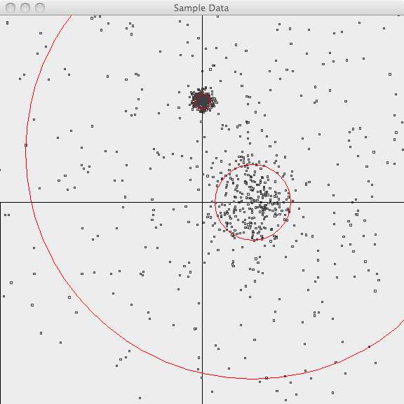
The following images illustrate Canopy clustering applied to a set of
randomly-generated 2-d data points. The points are generated using a normal
distribution centered at a mean location and with a constant standard
deviation. See the README file in the /examples/src/main/java/org/apache/mahout/clustering/display/README.txt
for details on running similar examples.
The points are generated as follows:
- 500 samples m=[1.0, 1.0](1.0,-1.0.html)
sd=3.0
- 300 samples m=[1.0, 0.0](1.0,-0.0.html)
sd=0.5
- 300 samples m=[0.0, 2.0](0.0,-2.0.html)
sd=0.1
In the first image, the points are plotted and the 3-sigma boundaries of
their generator are superimposed.
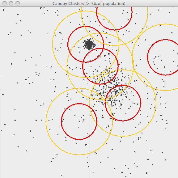
In the second image, the resulting canopies are shown superimposed upon the
sample data. Each canopy is represented by two circles, with radius T1 and
radius T2.
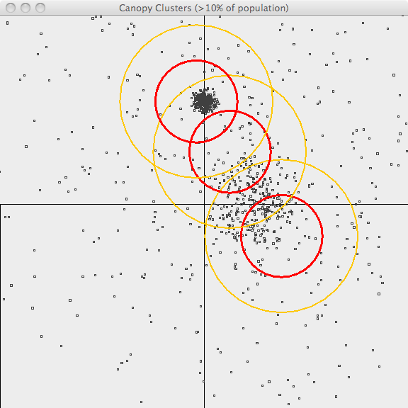
The third image uses the same values of T1 and T2 but only superimposes
canopies covering more than 10% of the population. This is a bit better
representation of the data but it still has lots of room for improvement.
The advantage of Canopy clustering is that it is single-pass and fast
enough to iterate runs using different T1, T2 parameters and display
thresholds.
Parameters
| Parameter |
Description |
Default Value |
'distanceMeasure |
The metric used for calculating distance, see Distance Metrics |
'Cosine |
't1 |
The "loose" distance in the mapping phase</code> |
0.5 |
't2 |
The "tight" distance in the mapping phase</code> |
0.1 |
't3 |
The "loose" distance in the reducing phase</code> |
't1 |
't4 |
The "tight" distance in the reducing phase</code> |
't2 |
Example
val drmA = drmParallelize(dense((1.0, 1.2, 1.3, 1.4), (1.1, 1.5, 2.5, 1.0), (6.0, 5.2, -5.2, 5.3), (7.0,6.0, 5.0, 5.0), (10.0, 1.0, 20.0, -10.0)))

import org.apache.mahout.math.algorithms.clustering.CanopyClustering

val model = new CanopyClustering().fit(drmA, 't1 -> 6.5, 't2 -> 5.5, 'distanceMeasure -> 'Chebyshev)
model.cluster(drmA).collect